6 Epistemology, Probability, and Science
Jonathan Lopez
Chapter Learning Outcomes
Upon completion of this chapter, readers will be able to:
- Distinguish between formal and traditional epistemology, including their main characteristics, motivations, and assumptions.
- Cultivate an intuitive sense of how basic formal methods apply to everyday thinking and decision-making.
- Employ Bayesianism in scientific contexts, specifically for hypothesis testing.
- Evaluate the strengths and limitations of Bayesianism.
Preamble
Epistemologists have traditionally approached questions about the nature of knowledge and epistemic justification using informal methods, such as intuition, introspection, everyday concepts, and ordinary language. [1] Whether in addition to or in place of these methods, formal epistemology utilizes formal tools, such as logic, set theory, and mathematical probability. The upshot is greater precision, increased rigor, and an expanded range of applications. This chapter focuses on the formal approach in its most prominent manifestation: Bayesianism, which begins by discarding the traditional view of belief as an all-or-nothing affair (either you believe a proposition or you don’t) and instead treats belief as admitting of degrees. These degrees are governed by how strongly a proposition is supported by the evidence. Evidential support is measured by probability, especially with the help of a famous result in probability theory, Bayes’s theorem (hence the term, “Bayesian”). Our aim here is to understand the basics of Bayesianism, its pros and cons, and an extended application to the epistemology of science. As we’ll see, the Bayesian framework is a natural fit for the scientific context. Very seldom does a single experiment change the opinion of the scientific community; the quest for scientific truth is hard fought over many experiments and research programs as hypotheses gradually gain or lose favor in light of a changing body of evidence. Bayesianism allows us to model this process, come to a more robust understanding of scientific knowledge, and use this understanding to settle some controversies over theory choice.
Degrees of Belief
You are probably more confident in some beliefs than others. You’ve probably said things like “I’m [latex]100\%[/latex] sure I turned the oven off,” which is to say your confidence is high, or “I have a hunch he might not be telling the truth,” which is to say your confidence is low. When you closely scrutinize your beliefs, you’ll find that they fall along various points in a spectrum—a hierarchy which can’t be captured simply by saying that you either believe or you don’t. Such all-or-nothing terms lump beliefs together into broad categories, masking important differences among their locations in the hierarchy.
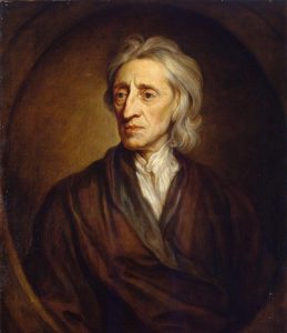
Suppose instead you understand belief as “admitting of degrees.” This allows you to distinguish beliefs in which you have varying degrees of confidence: your degree of belief in a proposition is the degree of confidence you have in that proposition, which can be placed on a scale from [latex]0[/latex] to [latex]1[/latex] (expressed in decimal, ratio, or percentage form)[2]. A belief that has accrued significant evidential support receives a high “score” or degree, which would gradually diminish with decreasing support. Plausibly, the all-or-nothing standards of traditional epistemology can then be mapped onto degreed terms according to a thesis named after British philosopher John Locke (1632–1704):
The Lockean thesis: A belief (in the all-or-nothing sense) is rational when the rational degree of belief is sufficiently high (i.e., above some specific threshold). (Foley 1992) [3]
Given this thesis, an advantage of the degreed framework is that it provides the resources to distinguish and evaluate specific levels of belief in a way that also grounds the traditional epistemological standards. In what follows, we will focus on the degreed aspects, keeping in mind that translation back into traditional terms is always possible via the Lockean thesis.
Formal epistemologists often talk about degrees of beliefs as credences. For example, take the statement, “All bachelors are unmarried,” which is analytically true (true by definition) and therefore impossible to be false. [4] A credence of this caliber would receive a perfect score of [latex]\dfrac{100}{100} = 100\% = 1[/latex]. Such a score represents absolute certainty. Just short of this are beliefs that are nearly certain but can, theoretically, be mistaken. For example, you’re probably nearly certain that the external world exists, although there’s a slight chance that you’re actually a brain in a vat and your experience of the world is being simulated. [5] If so, you have a really high credence, perhaps [latex]\dfrac{95}{100} = 95\% = 0.95[/latex], that you are not a brain in a vat. The further removed from absolute certainty, the lower the score a belief would receive. A score of [latex]0[/latex] is reserved for beliefs that can’t possibly be true, often because they are analytically false (self-contradictory)—for example, “The number [latex]42[/latex] is both even and odd.” This framework can make sense of statements like “I’m [latex]100\%[/latex] sure I set the alarm” and “There is a [latex]0\%[/latex] chance I’m getting that job” (perhaps after a bad interview). However, these sentences would, strictly speaking, be hyperbole, since they are neither tautologies nor contradictions—just highly likely and highly unlikely, respectively. There are, of course, slight leanings—propositions you barely believe or weakly reject. And in the middle, at [latex]\dfrac{50}{100} = 50\% = 0.5[/latex] credence, there are propositions on which you probably suspend judgment (have no opinion on one way or another), for example “The total number of people currently living on Earth is odd rather than even.” [6]
Two Models of Degrees of Belief
The best way to understand how “scores” are assigned to beliefs depends on whom you ask and what your purposes are. The previous section treated credences as values on a scale from [latex]0[/latex] to [latex]1[/latex]. This scale aligns them with how we typically think of probabilities, which also fall between [latex]0[/latex] and [latex]1[/latex] according to a standard axiom of probability theory:
The probability of a proposition or event [latex]X[/latex], represented by [latex]P(X)[/latex], is such that: [latex]0 \le P(X) \le 1[/latex].
More generally, formal epistemologists typically adopt probabilism: the view that credences should conform to probabilities. A significant upshot is that we can use the advantages of probability theory to talk and reason carefully about our beliefs. However, there are two ways to think about probability, which correspond to two ways to think about degrees of belief: objective and subjective.
An objective understanding of degrees of belief understands the “score” we’ve been talking about as a feature of the real (external, mind-independent) world. For example, if I asked for your degree of belief in a fair coin coming up heads, you’d likely say [latex]1[/latex] in [latex]2[/latex], or [latex]50\% = 0.5[/latex]. This is grounded in the fact that the coin has one side that is heads (the desired outcome) out of the two possible outcomes for a single toss. Getting a royal flush in poker follows the same reasoning with larger numbers: there are four ways to do it out of [latex]2,598,960[/latex] possible poker hands ([latex]1[/latex] in [latex]649,740[/latex]). In general, the objective probability, hence the objective degree of belief one should have, is equal to the number of ways the desired outcome can obtain out of the number of all relevant possible outcomes:
[latex]P(X) =\dfrac{\text{# of ways X can obtain}}{\text{Total # of relevant possible outcomes}}[/latex]
The denominator of this ratio is the size of the reference class (the set of all relevant possible outcomes). [7] In the coin case, the reference class consists of two possible outcomes: heads and tails. In the card case, the reference class consists of all possible hands in a poker game. But matters aren’t always so clear-cut. For example, consider the event, “Your local sports team will win their next championship.” Would we consider all past and future games that the team has ever played? Should we only consider their past and future championship games? Of course, we can’t directly inspect future games at present. So, do we simply look at the past? If so, how far back should we go? Surely their victories and losses in the 1970s aren’t relevant to this year. Now consider what credence to assign a belief such as, “Napoleon’s conquest in Europe would have been successful had he never ventured into Russia during the winter.” Despite this being intuitively likely, it would be even harder here to decide where to start in assigning a reference class. This set of confusions is known as the reference class problem.
A subjective understanding of degrees of belief avoids this problem by not tying your belief to the nature of the event in question. On this understanding, the score one attributes to a belief is a subjective probability: how confident you actually are in that belief being true, regardless of any features of the real, mind-independent world. This allows you to say things like “I’m [latex]75\%[/latex] sure my friend is going to be late” and “I’m [latex]90\%[/latex] sure my local sports team will win their next championship” without deciding on a reference class to use in a ratio.
Although the subjective interpretation allows us to expand the class of events or propositions we can sensibly assign probabilities to, it invites a host of other problems. One of the most prominent problems for the subjective understanding is the problem of the priors (the name for which will become apparent in the next section). Basically, if your subjective probabilities aren’t grounded in anything in the real world, they are just up to each individual person. Does this mean anyone can just set their subjective probabilities to whatever they want? Well, they could, but there are at least some constraints on what makes a set of subjective probabilities rational.
As with your beliefs in a traditional (non-degreed) framework, credences should not violate the laws of logic. For example, you shouldn’t believe two propositions that contradict each other. The degreed framework additionally requires us to respect the laws of probability.
Let’s say you decide to try out your hand at the racetrack and, as luck would have it, show up the day they’re racing Corgis (a Welsh dog breed). Before the races begin, you get to meet some of the racers. The first Corgi, Atticus, has cute little legs, is a little on the chubby side, but has a smile that convinces you that he will win the race. You decide he has an [latex]80\%[/latex] chance. The next Corgi you meet, Banquo, is half German Shepherd, is much taller and leaner, and hasn’t stopped staring into the middle distance in a determined fashion. You are now convinced that Banquo will win with a credence of [latex]80\%[/latex]. After meeting all the racers, and subsequently falling in love with all of them, you want everyone to win and therefore assign each a probability of [latex]80\%[/latex]. Assigning every contestant such a high probability is irrational. But why, especially on the subjective understanding?
A way to test whether any of your probabilities are irrational in the degreed framework is analogous to how you might evaluate beliefs in a non-degreed framework: you check for inconsistencies. In a non-degreed framework, the inconsistencies come in the form of logical contradictions among beliefs. In the degreed framework, inconsistencies arise when the probabilities you attribute to beliefs don’t respect the laws of probability (along with the laws of logic). One such law, finite additivity, maintains that if two propositions or events, [latex]X[/latex] and [latex]Y[/latex], are incompatible, their probabilities must be additive (the sum of their individual probabilities):
[latex]P(X\text{ or }Y) = P(X) + P(Y)[/latex], where [latex]X[/latex] and [latex]Y[/latex] cannot both obtain.
An example of incompatible events is a normal coin landing both heads, [latex]H[/latex], and tails, [latex]T[/latex], on a single toss. Setting aside the negligible possibility of the coin landing on the edge, [latex]H[/latex] and [latex]T[/latex] each has a probability of [latex]\dfrac{1}{2}[/latex]. So, finite additivity implies that [latex]P(H\text{ or }T) = P(H) + P(T) = \dfrac{1}{2}+\dfrac{1}{2} = 1[/latex]. In other words, the probability that either [latex]H[/latex] or [latex]T[/latex] obtains is [latex]1[/latex], or certainty.
Return to the racing example. You can discover that assigning an [latex]80\%[/latex] subjective probability to all the racers is irrational if you are forced to “put your money where your mouth is.” Table 1 summarizes the pertinent information you would see displayed at a betting counter. The racetrack assigns each racer betting odds, which can be translated into the probability of winning.
| Racer | Betting Odds ([latex]A\text{ to }B[/latex]). You stand to gain [latex]$A[/latex] (the amount the bookie puts up) for every [latex]$B[/latex] you bet. |
Probability of Winning = [latex]\dfrac{B}{(A+B)}[/latex] | Expected Payout per [latex]$1[/latex] Bet = [latex]\dfrac{(A+B)}{B}[/latex] |
|---|---|---|---|
| Atticus | [latex]4\text{ to }1[/latex] | [latex]20\%[/latex] ([latex]\dfrac{1}{5}[/latex]) | [latex]$5[/latex] |
| Banquo | [latex]1\text{ to }1[/latex] | [latex]50\%[/latex] ([latex]\dfrac{1}{2}[/latex]) | [latex]$2[/latex] |
| Cheddar | [latex]4\text{ to }1[/latex] | [latex]20\%[/latex] ([latex]\dfrac{1}{5}[/latex]) | [latex]$5[/latex] |
| Dr. Waddle | [latex]9\text{ to }1[/latex] | [latex]10\%[/latex] ([latex]\dfrac{1}{10}[/latex]) | [latex]$10[/latex] |
For example, since Banquo is the favorite to win the race, the racetrack gives him “even odds” ([latex]1\text{ to }1[/latex]) to avoid paying out very much money. Atticus, though adorable, is less likely to win, so the racetrack gives him [latex]4\text{ to }1[/latex] odds. Dr. Waddle, the least likely to win, will pay off the most if he can pull off the upset at [latex]9\text{ to }1[/latex]. The way to read these betting odds is to understand them as hypothetical amounts that the bookie and yourself, respectively, put up. This means that if Atticus wins, you’ll receive the [latex]$4[/latex] the bookie bet and get back the [latex]$1[/latex] you bet. You can, of course, bet whatever quantity you desire. The betting odds simply set the ratio.
If a bookie overheard you saying all the Corgis are likely to win, with an [latex]80\%[/latex] chance each, she could try to take advantage of this by offering you the revised set of bets summarized in Table 2 below. The bookie arrived at her numbers using the same strategy as the racetrack. If you accept, as your credences suggest, you will be guaranteed to lose money. It will cost you [latex]$4[/latex] to place bets on all the Corgis, but you will get back just [latex]$1.25[/latex] since only one Corgi will actually win.
| Racer | Subjective Probability of Winning | Betting Odds You Should Accept (Given Your Subjective Probabilities) |
Expected Payout per [latex]$1[/latex] Bet |
|---|---|---|---|
| Atticus | [latex]80\%[/latex] | [latex]1\text{ to }4[/latex] | [latex]$1.25[/latex] |
| Banquo | [latex]80\%[/latex] | [latex]1\text{ to }4[/latex] | [latex]$1.25[/latex] |
| Cheddar | [latex]80\%[/latex] | [latex]1\text{ to }4[/latex] | [latex]$1.25[/latex] |
| Dr. Waddle | [latex]80\%[/latex] | [latex]1\text{ to }4[/latex] | [latex]$1.25[/latex] |
Another way to put the fact that you are guaranteed to lose is that you have had a Dutch book made against you. To avoid Dutch books, you need to adjust your credences to align with the laws of probability. It is rational to avoid Dutch books. So, according to the Dutch book argument, rational credences adhere to the laws of probability (Vineberg 2016).
Though the Dutch book argument begins to make subjective probability more palatable by placing some firm constraints on the probabilities you can rationally assign, some would object that these constraints are too demanding. This objection to probabilism in general (whether objective or subjective) is the problem of logical omniscience. At the beginning of the chapter, it was mentioned that all and only necessary truths, such as those of logic (e.g., [latex]\textit{p}[/latex] or [latex]\text{not-}\textit{p}[/latex] ), deserve a perfect score of [latex]1[/latex]:
[latex]P(X) = 1[/latex] when [latex]X[/latex] is necessarily true
and
[latex]P(X) = 0[/latex] when [latex]X[/latex] is necessarily false.
However, there are an infinite number of logical truths. Since human beings (individually and collectively) are finite, there are many logical truths that no person has ever thought about. Some of them are beyond our limited grasp, since there is no limit to how complex they can be. Even many simple logical truths aren’t recognized without studying logic. For a number of reasons, then, no human has the capacity to form a belief in every logical truth, making it impossible for us to assign [latex]1[/latex] to them all. By adopting the degreed framework, we are committed to saying our beliefs behave in accordance with the laws of logic and probability. But if there are many instances where they don’t, as we seem to have found, we should rethink this relationship.
In response, we might say that the laws of logic and probability are nevertheless standards for ideal rational agents , which can be viewed as a kind of theoretical limiting case for those of us in the messy real world. In this approach, we are engaging in idealization much like physicists do when they reason with their frictionless planes, complete vacuums, and perfect spheres. Still, the Dutch book argument doesn’t stop people from having ridiculous credences so long as they respect the laws of probability. Almost any credence (e.g., that your local sports team is [latex]99.9\%[/latex] likely to win the championship) can be made probabilistically consistent with other credences if they are adjusted to fit. Objective probability could appeal to features of the real world to settle the appropriate credence, but subjective probability does not have this advantage. We will return to this problem for subjective probabilism in the final two sections to see if it can be mitigated.
Bayes’s Theorem and Bayesianism
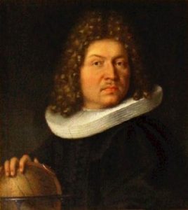
The previous sections introduced some of the critical ingredients for using Bayes’s theorem, a powerful theorem in probability theory established by Reverend Thomas Bayes (ca. 1702–1761). This theorem gives you the rules to follow to update your credences based on incoming evidence. Bayesianism is a version of formal epistemology that gives Bayes’s theorem a central role in updating credences. After all, not just any way of updating is rational. For example, after watching a couple of news reports about airplane crashes in the same week, you might be tempted to lower your credence that air travel is safe to the point that you’re afraid to fly. Decreasing your degree of belief in the safety of air travel to this extent would be irrational because the evidence isn’t strong enough. After all, think of all the safe flights that occur on a regular basis compared to those that crash. To see how we might approach updating your belief in a rational way, let’s look at the components of Bayes’s theorem.
Bayes’s theorem is often stated as follows:
[latex]P(H|E) = \dfrac{P(E|H) \cdot P(H)}{P(E)}[/latex], where [latex]P(E) \neq 0[/latex].
[latex]P(H|E)[/latex] represents the probability of a hypothesis [latex]H[/latex] given evidence [latex]E[/latex], where [latex]H[/latex] and [latex]E[/latex] are any two propositions or events. It tells you how likely [latex]E[/latex] makes [latex]H[/latex]. Because this probability is dependent or conditional on [latex]E[/latex], it is referred to as a conditional probability.
The process of obtaining this probability is called conditionalization (or conditioning). Prior to conditionalization, one begins with a prior probability, [latex]P(H)[/latex]. This is a kind of baseline or starting probability for [latex]H[/latex], one that does not yet take evidence [latex]E[/latex] into account. After conditionalizing, one ends up with a posterior probability, [latex]P(H|E)[/latex].
Given these concepts, we are now in a position to understand the rule of conditionalization, which is a relatively intuitive proposal: whenever a person gains new evidence [latex]E[/latex] concerning hypothesis [latex]H[/latex], the proper way to update one’s initial credence in [latex]H[/latex]—given by [latex]P(H)[/latex]—is by conditionalizing on [latex]E[/latex], then conforming one’s new credence to the result: [8]
After gaining evidence [latex]E[/latex], the updated credence [latex]P_{new}(H)[/latex] is given by [latex]P(H|E)[/latex].
The importance of Bayes’s theorem is that it helps us put this into practice by giving us a precise means by which to calculate the effect of conditionalization. But before we can see how this works, we must first examine the other components of the theorem.
[latex]P(E|H)[/latex] is the probability of obtaining the evidence [latex]E[/latex] given that the hypothesis [latex]H[/latex] is true. This component is often called the likelihood. It is sometimes described as the “explanatory power” of [latex]H[/latex] with respect to [latex]E[/latex]. Basically, it measures how well your hypothesis predicts the evidence. If a properly conducted and well-designed experiment yields [latex]E[/latex] as the expected result of [latex]H[/latex], this value will be high.
[latex]P(E)[/latex] is the probability of obtaining evidence [latex]E[/latex]. If the evidence is easily obtained by chance, it would not be a good idea to increase your confidence in the hypothesis. Bayes’s theorem accounts for this because if [latex]P(E)[/latex] is large, it will decrease your posterior probability in virtue of being in the denominator of our calculations, rendering the ratio smaller.
Comparative Bayesianism
One way to use Bayes’s theorem is to calculate the right-hand expressions in the formula and plug in the values to get a number for [latex]P(H|E)[/latex], then update your credence accordingly. But sometimes it is difficult to find a value for [latex]P(E)[/latex]. We can bypass this by using the theorem in a comparative fashion. If we want to use [latex]E[/latex] to choose between two competing hypotheses [latex]H_{1}[/latex] and [latex]H_{2}[/latex], we only need to show that [latex]P(H_{1}|E) > P(H_{2}|E)[/latex]. Applying Bayes’s theorem to each side of the inequality, [latex]P(E)[/latex] will appear on both sides and cancel out. The result is that:
[latex]P(H_{1}|E) > P(H_{2}|E)[/latex] when [latex]P(E|H_{1})P(H_{1}) > P(E|H_{2})P(H_{2})[/latex].
And if we start out neutral between [latex]H_{1}[/latex] and [latex]H_{2}[/latex], so that [latex]P(H_{1}) = P(H_{2})[/latex], then those cancel too. The result is that:
[latex]P(H_{1}|E) > P(H_{2}|E)[/latex] when [latex]P(E|H_{1}) > P(E|H_{2})[/latex], for cases where [latex]P(H_{1}) = P(H_{2})[/latex].
In other words, given that all else is equal, we should adopt [latex]H_{1}[/latex] over [latex]H_{2}[/latex] when the former better explains or predicts the evidence. So comparative Bayesianism gives us a probabilistic verification of a form of inference to the best explanation.
Note that where we have only a single hypothesis [latex]H[/latex], we can still use the above comparative formulation to compare [latex]H[/latex] to [latex]\text{not-H}[/latex] (by substituting [latex]H[/latex] for [latex]H_{1}[/latex] and [latex]\text{not-H}[/latex] for [latex]H_{2}[/latex]):
[latex]P(H|E) > P(\text{not-H}|E)[/latex] when [latex]P(E|H) > P(E|\text{not-H})[/latex], for cases where [latex]P(H) = P(\text{not-H}) = \dfrac{1}{2}[/latex].
But we must be cautious not to drop out the [latex]P(H)[/latex] in this way—except when comparing [latex]H[/latex] with another hypothesis that is equally likely. In other cases, [latex]P(H)[/latex] can have a dramatic impact on the calculation. In fact, ignoring prior probabilities and focusing exclusively on the conditional probabilities is the notorious base-rate fallacy (so named because [latex]P(H)[/latex] is sometimes called the base rate). Psychologists have identified this fallacy as a common source of many real-world reasoning mistakes, ranging from medical misdiagnoses to legal errors to discriminatory policies (Kahneman and Tversky 1973). To get a sense of how this fallacy operates in the medical context, try your hand at question 2 in the Questions for Reflection at the end of this chapter.
Box 1 – Ockham’s Razor
Ockham’s razor, which posits that “entities should not be multiplied beyond necessity,” serves as a guiding principle for choosing among competing hypotheses. The core insight is that we should stick to the simplest explanation consistent with the data, ensuring that any additional postulates aren’t superfluous. Since simplicity is an explanatory virtue (among others)—that is, it improves the quality of an explanation (other things being equal)—Ockham’s razor is closely related to inference to the best explanation.
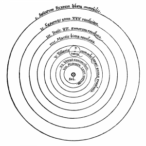
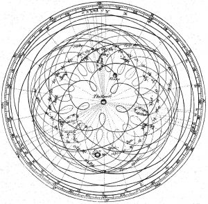
The choice between a heliocentric or geocentric model of the universe shows how “the razor” plays out in a scientific context. The heliocentric model of the universe maintains that the planets orbit the sun. The geocentric model maintains that they orbit Earth. However, to account for observations, the geocentric model further stipulates that the planets exhibit “epicycles,” meaning that they move backward and forward via smaller loops within their orbits. These epicycles may be seen as an extra entity or postulate. Although the razor doesn’t eliminate the postulate with certainty , it renders the geocentric model less probable than the heliocentric model .
Adding a new entity/postulate is equivalent to adding a conjunct (an “and”) to the hypothesis, which (because of how probabilities are calculated) only works to drive down one’s credence. Mathematically, we can express this as the following probabilistic law:
[latex]P(X\text{ and }Y) < P(X)[/latex] when [latex]\text{X}[/latex] does not entail [latex]\text{Y}[/latex].
Consider the following example made famous by psychologists Kahneman and Tversky (1983). Linda is a recent university grad who studied philosophy. While at university, Linda regularly participated in activism related to racial injustice and climate change. Which is more probable?
- Linda is a bank teller.
- Linda is a bank teller and is active in the feminist movement.
If you’re like most people, you will likely have chosen (b). However, (b) is the less likely option because no matter what probabilities you assign to each attribute—“bank teller” and “active in the feminist movement”—it will always be less likely for both attributes to appear together rather than either on its own. For an extended explanation and discussion of this example, see Berit Brogaard (2006). For more on Ockham’s razor, see Elliott Sober (2015 and 2016).
Application: The Epistemology of Science
Revising your credence in a hypothesis in response to evidence, specifically, empirical observations, is what science is all about. One of the reasons Bayesianism has been so influential is that it generalizes across many fields and scenarios. In this section, we will look at how one might use Bayesianism to assist in updating degrees of belief in scientific hypotheses.
Suppose you want to know whether vaccines cause autism, so you set out to do some research. After a half hour on Google, you find yourself in a vortex of misinformation. You come across the (in)famous 1998 Lancet article responsible for instigating the vaccine/autism misconception. In this article, Dr. Andrew Wakefield and his co-authors report a study in which [latex]8\text{ of }12[/latex] children showed the onset of behavioral symptoms associated with autism within weeks of receiving the measles, mumps, rubella (MMR) immunization. On this basis, you accept an [latex]\dfrac{8}{12} \approx 66.67\%[/latex] chance that vaccines cause autism, and form an [latex]\approx 0.667[/latex] credence that your child will develop autism [latex](H)[/latex] if you let her receive the immunization [latex](E)[/latex]. In other words, your initial estimate is that [latex]P(H|E) \approx 0.667[/latex]. However, you then learn that The Lancet retracted the article after the study had been repeatedly discredited. While anti-vaxxers continue to side with Wakefield, others insist that vaccines are safe and vital to public health.
What should you do? Determined to sort this out but unsure of your probability skills, an intriguing open textbook chapter about Bayesian epistemology catches your eye. Equipped with your new knowledge of Bayes’s theorem, you seek out some experiments to obtain the probabilities to input into the theorem. Fortunately, there are many such experiments to draw from. As an example, consider just one study done in Quebec (Fombonne et al. 2006).
The study reports that [latex]\approx 65\text{ per }10,000[/latex] children were diagnosed with a condition on the autism spectrum. So, [latex]P(H) \approx \dfrac{65}{10000} = 0.0065[/latex]. The researchers report that this is consistent with the [latex]0.6\%[/latex] rate found in other epidemiological studies. They also calculate an average [latex]93\%[/latex] vaccination rate among children in the relevant age group, which yields [latex]P(E) = 0.93[/latex]. If vaccines cause autism, one might expect a higher-than-normal vaccination rate concentrated among the [latex]65[/latex] diagnosed with autism. To give anti-vaxxers the benefit of the doubt, suppose that [latex]64\text{ of the }65[/latex] (about [latex]98\%[/latex]) were immunized. That is, [latex]P(E|H) ≈ 0.98[/latex].
Using Bayes’s theorem,
[latex]P(H|E)=\dfrac{P(E|H) \cdot P(H)}{P(E)}\approx\dfrac{0.98\cdot(0.0065)}{0.93}\approx0.0068=0.68\%[/latex]
Putting it all together, this result suggests that the rational response to the evidence is to dramatically downgrade your credence in the hypothesis from the initial [latex]66.67\%[/latex] to less than [latex]1\%[/latex]. While we might not ever fully rule out the hypothesis, additional experiments could continue this downward slope until credences become vanishingly small. Even at [latex]1\%[/latex], you would already be justified in believing that it is highly improbable that vaccines cause autism—in other words, justified in believing that it is highly probable ([latex]99\%[/latex]) that vaccines do not cause autism. A corollary to this is that no matter how much evidence accrues, you will never be able to raise your credence to [latex]1[/latex], or absolute certainty. This point generalizes: a Bayesian treatment of science best accords with fallibilism, the idea that one can have justification without certainty.
Our example also demonstrates that Bayesianism has some mechanism for correcting prior probabilities, since enough evidence will wash out erroneous priors. One might appreciate that we could have started off skeptical about the claim that vaccines cause autism, say with [latex]5\%[/latex] confidence, and our credence would still have decreased after seeing the evidence. In the short term, however, subjective Bayesianism would allow someone to believe in unrealistic priors until enough evidence comes in. Objective Bayesianism has the advantage on this front because it insists on having priors that cohere with the world before one gets on with the business of updating (though on the other hand, the objective view faces the reference class problem).
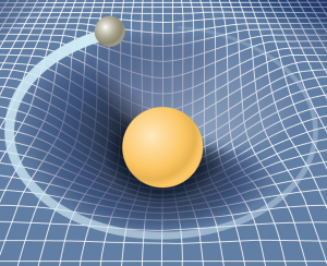
The vaccine case required us to appeal to observed rates and statistical calculations to determine the probabilities to input into Bayes’s theorem. However, it’s not always possible to put a number on the relevant values. Consider Einstein’s theory of general relativity, which postulates that mass causes spacetime to warp or curve, and that this curvature is the force of gravity. At the time of its publication in 1915, most scientists viewed this theory as a radical, unwarranted departure from the longstanding Newtonian theory of gravity. After all, Einstein had no empirical proof. On the other hand, his reasoning also seemed convincing, not to mention that he had been proved right once before when everyone else had it wrong (regarding his theory of special relativity in 1905). So, in 1915, it was perhaps reasonable to form a [latex]\dfrac{50}{50}[/latex] credence on the question of Newtonian gravity ([latex]N[/latex]) vs. general relativity ([latex]GR[/latex]). If so, then [latex]P(N) = P(GR)[/latex].
Whereas [latex]N[/latex] predicts that light rays approaching the sun would travel a straight path, [latex]GR[/latex] predicts that they would be warped by the sun’s gravity, taking a curved path. During the total solar eclipse in 1919, the famous Eddington experiment ([latex]E[/latex]) strongly confirmed [latex]GR[/latex]’s prediction. In other words, [latex]P(E|GR) >> P(E|N)[/latex], where the double inequality means “much greater than.” Of course, it’s hard to see how numerical values could be determined.
Comparative Bayesianism to the rescue! Given what we just determined—that [latex]P(N) = P(GR)[/latex] and [latex]P(E|GR) >> P(E|N)[/latex]—the comparative version of Bayes’s theorem introduced in the previous section implies that [latex]P(GR|E) >> P(N|E)[/latex]. Hence, [latex]E[/latex] strongly supports [latex]GR[/latex] over [latex]N[/latex]. Comparative Bayesianism tells us that after we learn Eddington’s results, we should significantly increase our credence in [latex]GR[/latex] and decrease our credence in [latex]N[/latex]. Since those credences were previously equal, this means we will end up with [latex]P(GR|E) >> \dfrac{1}{2}[/latex]. In other words, we should strongly believe [latex]GR[/latex] over [latex]N[/latex].
Of course, this conclusion is somewhat limited. Without numerical probabilities, Bayesianism cannot pinpoint a specific degree of belief in [latex]GR[/latex]. Instead, comparative Bayesianism showed us how we are justified in choosing between two competing hypotheses. Further, comparisons can also usefully justify a “belief ranking” (e.g., belief [latex]B1[/latex] is more probable than [latex]B2[/latex], which is more probable than [latex]B3[/latex]). Decision theorists use such rankings to explain which beliefs should be given greater weight in decision-making.
Evaluating Bayesianism
This chapter has demonstrated that Bayesianism provides us with a strong supplement or alternative to traditional epistemology. A degreed framework allows us to characterize our doxastic attitudes more precisely. The tools of probability avail us to a rich mathematical framework for evaluating credences. The most valuable of these tools is Bayes’s theorem, which meticulously prescribes how to refine our credences over time in light of new evidence. The result is a powerful framework, one which can provide a strong epistemological ground for scientific inquiry.
This chapter has also shown that Bayesianism is not without its weaknesses, including the reference class problem, the problem of the priors, and the problem of logical omniscience. These, however, may not be insurmountable and are, in fact, the hub of lively debate and research in formal epistemology. Though this chapter focuses on examples from science, it might be appreciated that the result is highly generalizable. If you are intrigued by the potential of Bayesianism, it would be fruitful to look through the suggested reading list to understand how it makes contact with other areas of philosophy.
Questions for Reflection
- Create a sketch of what your own range of credences might look like. Use the continuum below to plot your credences for the propositions listed in (a)–(e). There are several benchmarks in the diagram to help guide your thinking.
- The scientific consensus is wrong about climate change.
- A nuclear strike will happen within your lifetime.
- Someone on a given crowded bus ([latex]\approx 30[/latex] passengers) has the same birthday as you.
- The final match of the next World Cup (soccer) will feature at least one European country.
- The Talking Heads (a rock band) will reunite for one final album.

- Let’s explore Bayes’s theorem and how it compares to your probability intuitions. Consider two claims:
[latex]T[/latex] = You test positive for a given medical condition.
[latex]C[/latex] = You have the medical condition.
Suppose the test has a strong track record for detecting the condition when it’s actually present: [latex]P(T| C) = 0.8[/latex]. Also suppose about [latex]1\%[/latex] of the population has the condition: [latex]P(C) = 0.01[/latex]. Finally, suppose about one of every ten people who are tested tend to test positive: [latex]P(T) = 0.1[/latex]. Now answer the following questions:- Using only your intuition (no calculations), how likely is it that you have the condition given that you tested positive? In other words, is [latex]P(C | T)[/latex] is high, low, or roughly in the middle?
- Now plug the numbers into Bayes’s theorem to find a numerical estimate for [latex]P(C | T)[/latex].
- Compare your answers to (a) and (b). If you found your intuition to be far off course, what do you think is the reason for this? What led your intuition astray? Were you selectively focused on one particular aspect of the provided data? Is the error related to the base-rate fallacy (introduced in the Comparative Bayesianism section)?
- Find your own example to demonstrate the use of comparative Bayesianism. Begin with a specific scientific or philosophical hypothesis [latex]H[/latex] in which your initial credence is [latex]0.5[/latex]. Describe any single consideration [latex]E[/latex] that seems to have some relevance to [latex]H[/latex]. According to comparative Bayesianism, how should learning about [latex]E[/latex] alter your credence in [latex]H[/latex]? Explain step by step.
- Is Bayesianism the way our brains “naturally” update beliefs? AI (artificial intelligence) researchers have had tremendous success by using Bayesian inference to approximate some human capabilities. Does this suggest we might have stumbled upon the algorithm our brain has been using all along? (See the paper in the Further Reading section by Robert Bain, “Are Our Brains Bayesian?”)
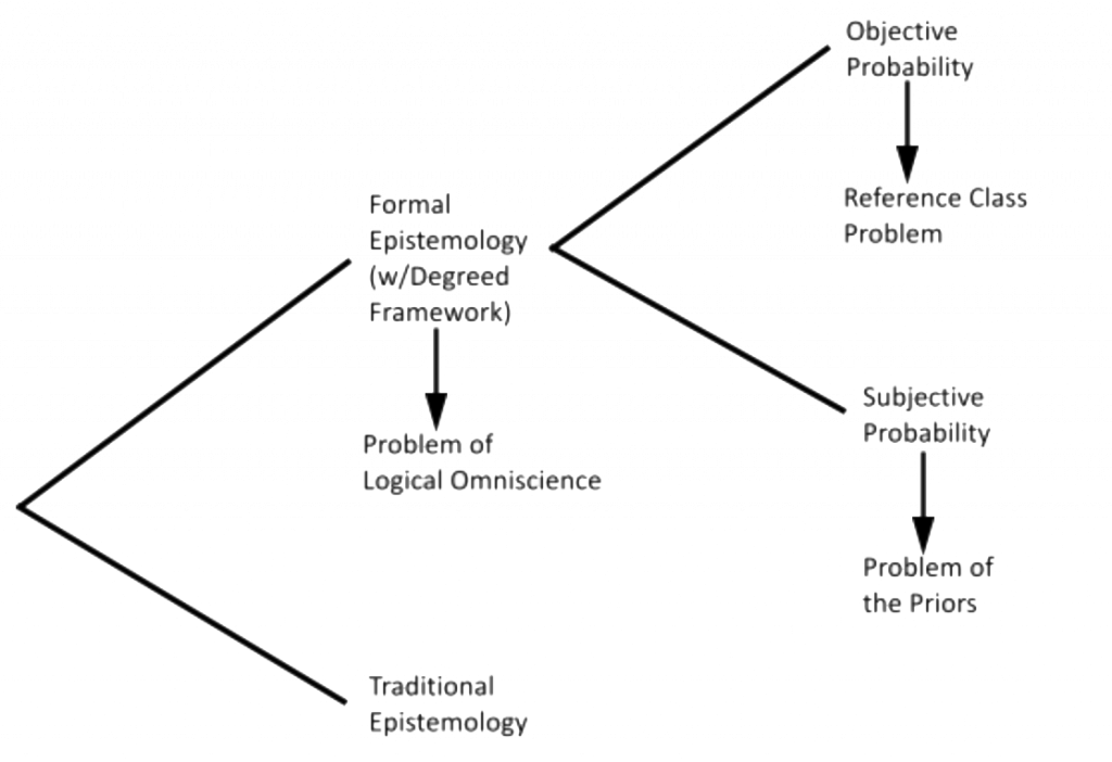
- Mapping Out the Terrain: Below is a roadmap of the epistemological terrain. Like most areas of philosophy, you will find yourself at a choice-point. Each option has pros and cons, but it’s up to you to defend your position whichever way you go. You’ve read about the upshots of the degreed framework, but it would be intellectually responsible to have something to say about the problems that each position inherits. As an exercise, determine which of the problems you think are the most serious and decide which position you think is most defensible, all things considered. Write a mini-essay explaining your decision.
- The House Always Wins: To get a better feel for Dutch books, it would be helpful to run through the following game. The example involves a roulette wheel, but for simplicity we will only consider bets that the ball will land on a number in the range [latex]1\text–36[/latex] and one of two green spaces ([latex]0[/latex] and [latex]00[/latex]), yielding a sample space (the set of all possible individual outcomes) of size [latex]38[/latex].
First consider what would happen if you place bets on all [latex]38[/latex] options. Although you will win some of these, since you covered all options, more of them will lose, guaranteeing a net loss. So, this is a Dutch book.
Now look instead at what happens when you repeat single bets in sequence. Suppose you start out with [latex]$200[/latex] and place [latex]$5[/latex] (minimum) bets on the simplified roulette wheel. First pick a number you wish to bet on. To see whether you won, use a random number generator to generate one number at a time with a range of [latex]1\text–38[/latex] and assume [latex]37[/latex] and [latex]38[/latex] stand in for the two green spaces ([latex]0[/latex] and [latex]00[/latex]), respectively. Then repeat. For each win, use the space in the table below to record your gain or loss. Though you might win once in a while, in the long run you will lose your entire initial pot of money. Try it and see how long it takes to reach that point.
| Event | Probability of Winning | Expected Payout per [latex]$5[/latex] bet | Your pot of money ( [latex]+$180[/latex] per win, [latex]-$5[/latex] per loss) Initial amount: [latex]$200[/latex] |
|---|---|---|---|
| [latex]0[/latex] | [latex]1\text { in }38\text{ }(\approx 2.78\%)[/latex] | [latex]$180\text{ }($36\times5)[/latex] | Remaining amount: ___ |
| [latex]00[/latex] | [latex]1\text { in }38\text{ }(\approx 2.78\%)[/latex] | [latex]$180[/latex] | Remaining amount: ___ |
| [latex]1\text–36[/latex] | [latex]1\text { in }38\text{ }(\approx 2.78\%)[/latex] | [latex]$180[/latex] | Remaining amount: ___ |
Further Reading
Basic Probability Theory
Brogaard, Berit. 2016. “‘Linda the Bank Teller’ Case Revisited.” Psychology Today (blog). November 22, 2016. https://www.psychologytoday.com/ca/blog/the-superhuman-mind/201611/linda-the-bank-teller-case-revisited .
Hacking, Ian. 2001. An Introduction to Probability and Inductive Logic, Chapter 6. New York: Cambridge University Press.
Metcalf, Thomas. 2018. “The Probability Calculus.” In 1000-Word Philosophy: An Introductory Anthology. https://1000wordphilosophy.com/2018/09/23/introduction-to-the-probability-calculus/ .
Philosophy of Probability
Metcalf, Thomas. 2018. “Interpretations of Probability.” In 1000-Word Philosophy: An Introductory Anthology. https://1000wordphilosophy.com/2018/07/08/interpretations-of-probability/ .
Bayesian Epistemology
Carneades.org. 2014. “Bayesian Epistemology.” YouTube video, 3.02. December 14, 2014. https://www.youtube.com/watch?v=YRz8deiJ57E&list=PLz0n_SjOttTdIqlgDjdNFfLUFVrl5j1J4 .
Talbott, William. 2008. “Bayesian Epistemology.” In The Stanford Encyclopedia of Philosophy, edited by Edward N. Zalta. https://plato.stanford.edu/entries/epistemology-bayesian/ .
Explanatory Considerations Related to Bayesianism
Sober, Elliott. 2015. Ockham’s Razors: A User’s Manual. New York: Cambridge University Press.
———. 2016. “Why Is Simpler Better?” Aeon. https://aeon.co/essays/are-scientific-theories-really-better-when-they-are-simpler .
AI, Cognitive Psychology, and Bayesianism
Bain, Robert. 2016. “Are Our Brains Bayesian?” Significance 13 (4): 14–19. https://doi.org/10.1111/j.1740-9713.2016.00935.x .
References
Foley, Richard. 1992. “The Epistemology of Belief and the Epistemology of Degrees of Belief.” American Philosophical Quarterly 29 (2): 111–21.
Fombonne, Eric, Rita Zakarian, Andrew Bennett, Linyan Meng, and Diane Mclean-Heywood. 2006. “Pervasive Developmental Disorders in Montreal, Quebec, Canada: Prevalence and Links with Immunizations.” Pediatrics 118 (1): 139–50.
Hájek, Alan. 2007. “The Reference Class Problem Is Your Problem Too.” Synthese 156: 563–85.
Kahneman, Daniel, and Amos Tversky. 1973. “On the Psychology of Prediction.” Psychological Review 80: 237–51.
Moon, Andrew. 2017. “Beliefs Do Not Come in Degrees.” Canadian Journal of Philosophy 47 (6): 760–78.
Tversky, Amos, and Daniel Kahneman. 1983. “Extensional versus Intuitive reasoning: The Conjunction Fallacy in Probability Judgment,” Psychological Review 90 (4): 293–315.
Vineberg, Susan. 2016. “Dutch Book Arguments.” In The Stanford Encyclopedia of Philosophy, edited by Edward N. Zalta. https://plato.stanford.edu/entries/Dutch-book/ .
Wakefield, A.J., et al. 1998. “RETRACTED: Ileal-Lymphoid-Nodular Hyperplasia, Non-Specific Colitis, and Pervasive Developmental Disorder in Children.” The Lancet 351 (9103). https://www.thelancet.com/journals/lancet/article/PIIS0140-6736(97)11096-0/fulltext .
- Refer to Chapters 1–4 of this volume for the foundations of traditional epistemology. ↵
- Compare Moon (2017), who distinguishes degrees of confidence from degrees of belief. On his view, beliefs do not come in degrees. ↵
- Here we leave the threshold unspecified, since it is up for debate. ↵
- Refer to K. S. Sangeetha, Chapter 3 of this volume, for further elucidation of the connection between analyticity, possibility, and necessity. ↵
- See Daniel Massey, Chapter 4 of this volume, for this and related skeptical scenarios. ↵
- Some will make a distinction between suspending/withholding judgment and having no attitude toward a proposition (e.g., a proposition that one doesn’t grasp or has never thought about). If so, the former would be located in the middle of the confidence scale, whereas the latter would amount to being off the scale altogether. It is also worth noting that some epistemologists will identify withholding belief as a (possibly vague) range that includes 0.5. Belief would then correspond to the part of the scale beyond that range up to and including 1, whereas disbelief would correspond to the part of the scale preceding that range down to and including 0. ↵
- “Reference class” is sometimes applied only to statistical probabilities and a “frequentist” interpretation. But others have generalized the meaning in accordance with the way I am using the term here. See Hájek (2007). ↵
- Since the rule of conditionalization does not reflect any uncertainty we have about the evidence itself, some Bayesians replace this rule with a modification called “Jeffrey conditionalization,” named after the philosopher who proposed it, Richard Jeffrey (1926–2002). Refer to the further reading on Jeffrey conditionalization for more on this issue. ↵
The branch of epistemology that utilizes formal methods, such as logic, set theory, and probability.
The study of knowledge and justified belief within a degreed framework using formal methods, especially probability theory with emphasis on Bayes’s theorem.
A degree of confidence (or credence) that a person places in the truth of a proposition.
The thesis, named after John Locke, which relates the all-or-nothing rationality of traditional epistemology to the degreed framework as follows: a belief is rational when the rational degree of belief is sufficiently high (i.e., above some specific threshold level).
Degrees of belief.
The view that credences should conform to the laws of probability.
The kind of probability grounded in features of the real, mind-independent world.
The set of all possible outcomes relevant to determining a given objective probability. One calculates the probability of an event or proposition X by dividing the number of possible ways in which X can obtain by the size of the reference class.
The problem of determining a reference class in cases where there is no clear choice.
Probabilities that are grounded in a person’s degrees of confidence in propositions.
The objection that subjective Bayesianism places no rational constraint on priors (prior probabilities).
The law of probability stating that if two probabilities, P(A) and P(B), are mutually exclusive, the probability that either A or B obtains is the sum of their individual probabilities: P(A or B) = P(A) + P(B). In other words, P(A or B) is “additive.”
A set of bets that, when accepted, yields a guaranteed loss.
An argument showing that rational credences must adhere to the laws of probability (based on the premise that rationality requires avoiding Dutch books).
An objection to probabilism, according to which adherence to the laws of probability would require logical omniscience (knowledge of, or at least justified belief in, all logically necessary truths).
A formula in probability theory attributed to Reverend Thomas Bayes. The formula is used by Bayesians to describe how to update the probability of a hypothesis H given new evidence E:
P(H|E) = [{P(E|H) ∙ P(H)}/P(E)], where P(E) ≠ 0.
Typically written in the form P(A|B), it is the probability that A obtains given that B obtains.
The process of moving from an absolute probability, such as P(A), to a conditional probability, such as P(A|B). By doing so, one “conditionalizes on B.”
Typically written as P(H) in Bayes’s theorem, it is the probability of a hypothesis H before conditionalization on evidence. Bayesians take prior probabilities, or priors, to represent one’s initial degree of belief in H.
Typically written as P(H|E) in Bayes’s theorem, it is the result of conditionalizing a hypothesis H on an incoming piece of evidence E, read as “the probability of the hypothesis given the evidence.”
The rule that one’s prior probability must be updated in light of new evidence by conditionalizing on that evidence (via Bayes’s theorem, according to Bayesians).
Typically written as P(E|H) in Bayes’s theorem, it measures the degree to which hypothesis H predicts or explains the evidence E. It is sometimes referred to as the “explanatory power” of H with respect to E.
Given that all else is equal, one should choose the hypothesis that best explains the evidence. One form of this can be justified by a comparative use of Bayes’s theorem. It is closely related to Ockham’s razor.
Ignoring a prior probability (or base rate) when determining a posterior probability.
The methodological principle which maintains that given two competing hypotheses, the simpler hypothesis is the more probable (all else being equal). As the “razor” suggests, we should “shave off” any unnecessary elements in an explanation (“Entities should not be multiplied beyond necessity”). The principle is named after the medieval Christian philosopher/theologian William of Ockham (ca. 1285–1347). Other names for the principle include “the principle of simplicity,” “the principle of parsimony,” and “the principle of lightness” (as it is known in Indian philosophy).
A feature of a hypothesis that improves its quality as an explanation of the available data (other things being equal). An example of such a feature is simplicity, according to Ockham’s razor. By contrast, an explanatory vice is a feature of a hypothesis that reduces its quality as an explanation (other things being equal). If simplicity is an explanatory virtue, then unnecessary complexity in a hypothesis is the corresponding explanatory vice.
The view that justification does not entail truth.
A version of Bayesianism that allows credences to be represented and governed by subjective probabilities.
A version of Bayesianism that requires credences to be represented and governed by objective probabilities.
In probability theory, it is the total set of possible simple outcomes for an event. A reference class consists in subsets of the sample space.
